As the GEMOC Studio offer different engines that requires specific configurations, it currently offers one launch configuration per engine. The views offered when running or debugging a model may also vary depending on the execution mode and the engine kind.
In Section 1, “Execute a model”, you’ll learn how to start and stop a model execution. Additionally, some engine may also provide some dedicated control panels and views. Section 2, “Animate a model” presents how to enable or disable the animation. Section 3, “Debug a model” presents how to suspend the execution in order analyze the model during its execution. Thanks to the trace support, in GEMOC, this activity allows to go forward but also backward and analyze several dimensions of the runtime data.
As the GEMOC Studio offer different engines that requires specific configurations, it currently offers one launch configuration per engine. The views offered when running or debugging a model may also vary depending on the execution mode and the engine kind.
Run and debug are configured using the launch configuration. An example of configuration:
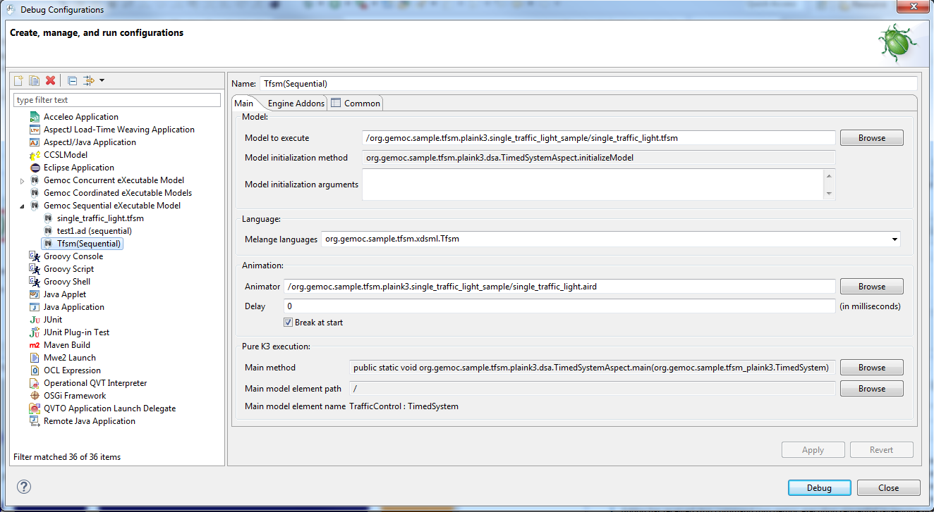
- Model to execute : this is the model that will be executed
- Model initialization method and argument : if the chosen language has a valid method with the
@InitializeModelannotation in its DSA, the field Model initialization method will be set and this method will be called before launching the animation. - Model initialization arguments : optional string arguments that can be passed to the initialization method. (one string per line)
- Melange languages : this field allows to select among the languages defined in Melange.
- Main method : the name of the method that can be used to start the engine. The possible value are specified by the language
designer in the language definition by adding an
@Mainannotation on methods in the DSA. - Main model element path : after having selected a main method, use the browse button to select a model element on wich this method will be called. This field presents its path in the model, the following field Main model element name displays a human readable name for this element.
The break at start tells to the debugger to add a virtual breakpoint on the first instruction that will run.
Note
@Main and @InitializeModel annotations used to declare possible methods used in this launcher are detailed in Section 1.1, “Defining the Domain-Specific Actions (DSA) Project for Sequential language”.
The run mode is the fastest way to execute a model. If an animation is defined, it will also be displayed (see Section 2, “Animate a model”). The execution cannot be paused/suspended. It can however be stopped. It offers a limited set of views :
- the Engine View allows to stop a running model.
- the MultiBranch Timeline View is displayed at the end of the execution in order to check the resulting execution trace.
If more feedback is required, please use one of the frontend or backend available for the xDSML, see Backends and frontends.
In debug mode, the engine offers more control over the execution. It allows to pause, add breakpoints, and execute the model in a step by step mode.
It reuses the Eclipse Debug perspective and some of its views and adds some Gemoc specific views.
- the Engine View allows to stop a running model.
- the Animation Manager View is displayed and updated in real-time during the simulation. It can display both an animation layer and a debug layer.
- the Debug View. This view presents an interface for Step by Step execution of the model.
- the Variable View. This view presents the Runtime Data as a (EMF based) tree.
When running a simulation in Debug mode, it is configured to activate automatically the Debug layer and the Animation layer in the Animation view.
On the engine addon tab, one can activate several optional addons.
- the MultiBranch Timeline View can be displayed during all the simulation.
- the MultiDimensional Timeline View can be displayed during all the simulation.
Run and debug are configured using the launch configuration. An example of configuration:
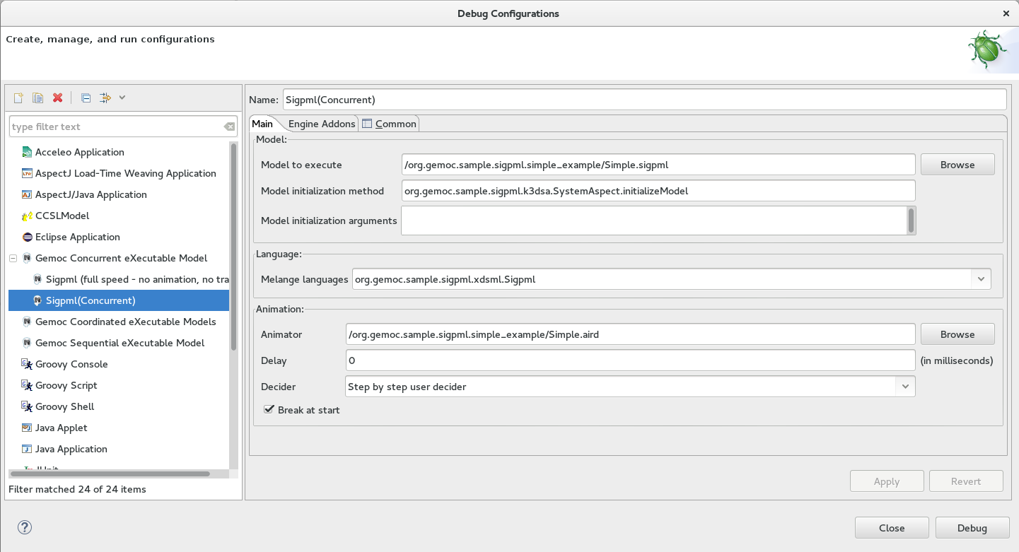
- Model to execute : this is the model that will be run
- Melange languages : this field allows to select among the languages defined in Melange.
-
Decider : this field allows to select the solver strategy used by the engine when several Logical Steps can be triggered. Possible choices are :
- Solver proposition : the solver internal strategy will be used to select a Logical Step
- Random : will randomly select one of the available Logical Step (warning: execution cannot be reproduced when using this Decider)
- Ask user : (available only in Debug mode), this option will use the Logical Step View or the MultiBranch Timeline View to present the available Logical Steps and pause if there are more than one Logical Step. The user will then need to click on one of the Logical Step to continue.
- Ask user (Step by step) : (available only in Debug mode), this option is similar to the previous one. However, it will pause on every Logical Step, even if there is only one Logical Step that can be triggered. This is more or less equivalent as putting a breakpoint on every MSE of the language.
More Deciders will be developed (for example for playing predefined scenario).
In run mode, it offers the faster way to run the model. It cannot be paused. However, you can stop it. It offers a limited set of views :
- the Engine View allows to stop a running model.
- the MultiBranch Timeline View is displayed at the end of the execution in order to control the resulting execution trace.
If more feedback are required, please use one of the frontend or backend available for the xDSML, see Backends and frontends.
In debug mode, the engine offers more control on the execution. It allows to pause, add breakpoint, and run in a step by step mode.
It reuses the Eclipse Debug perspective and some of its views and add some GEMOC specific views.
- the Engine View allows to stop a running model.
- the MultiBranch Timeline View can be displayed during all the simulation.
- the Logical Steps View is available for concurrent execution.
- the Stimuli Manager View is displayed during all the simulation.
- the Animation Manager View is displayed during all the simulation. It can display both an animation layer and a debug layer.
- the Debug View. This view presents an interface for Step by Step execution at the Logical Step level or even at the DSA level.
- the Variable View. This view presents the Runtime Data as a (EMF based) tree.
When running a simulation in Debug mode, it is configured to activate automatically the Debug layer and the Animation layer in the Animation view.
The break at start tells to the debugger to add a virtual breakpoint on the first instruction that will run.
GEMOC framework offer to language and/or engine developers the possibility to create Engine Addons (see Section 2.1, “Developing new Addons”). An Engine addon will connect to the running engine and all its data (model, context, etc) in order to provide new features to the end user who run a model (ie. model designer).
These addons may work in the background (for example for recording traces) but can also provide a graphical user interface.
These GUI can then provide dedicated backends or frontends views that respectively display informations from the running model or provide event input to the running model.
The activation or not of an addon is done in the Engine Addons tab.
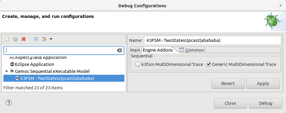
When selected, an addon (and its optional associated views) will be activated in both run and debug mode.
For example in Figure 16, “Selection of addons in the launch configuration tab”, selecting the a MultiDimentional Trace addon will enable the storing of the execution trace and thus allow to use the MultiDimentionnal timeline view. In this example, the user has the choice between the Generic MultiDimentional Trace addon and the language specific k3fsm MultiDimentional Trace addon (more efficient) generated thanks to the trace addon generator (see Section 1.3, “Defining MultiDimentional Trace support”).
Note
If most addons can be used for every languages, some addons may be developed for a single language or for a single engine.
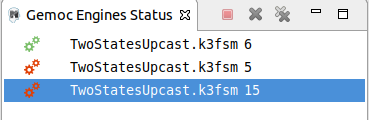
The engine view displays a list of execution engines and their status:
- current running status (Green = Running, Red = Stopped),
- number of steps that have been executed.
Note
The number of executed step shows only the steps that have finished. Ie. It is increased on step end. This means that in case of Step into nested calls, this number will increases only when it has finished the inner step.
Note
Timelines may choose to use they own step numbering and it may not be the same as the number of steps of this Engine view.
In Figure 17, “Engine View”, the buttons available on the top right of this view respectively allow to:
- Stop the selected engine (red square button)
- Remove/dispose the selected engine from the view (cross button) (the engine must be stopped)
- Remove/dispose all previously stopped engines from the view (crosses button)
Note
The Sirius diagram are not closed when the execution ends, they are closed only when the engine is disposed.
The CCSLJava engine adds some commands to the Engine view.
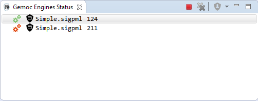
It adds a new button (represented as a shield on top right of Figure 18, “CCSLJava addition to Engine View”) that allows to change the current Logical Step decider used by the CCSLJava engine.
Tip
When running a model, You can easily "pause" the engine running with a solver or random decider by clicking on the change logical step decider (the shield button will be green when run in debug mode) this will automatically switch to the "Step by step decider". To restart, simply select back an automatic decider (solver or random) and select the next step in the LogicalStep view.
Warning
Even if they both pause the execution, choosing a "Step by step decider" is currently different from the "suspend" of a breakpoint from the Debug commands. The former ask the user for a decision about the logical step to execute and the later suspends the execution in order to analyze it.
Help is welcome to contribute a way to align them.
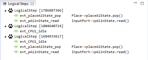
The Logical Step View is provided by the CCSLJava Engine.
The logical steps view displays the list of possible future executions. This list is provided by the solver. This view is organized around a tree. For each logical step, its underlying events can be seen and possibly for each event the associated operation is visible.
Note
This view displays nothing when execution runs in "run mode", per say this view is only of use when running in "debug mode".
The Stimuli Manager View is provided by the CCSLJava Engine.
The Stimuli Manager view display the list of MSE and has interactions with the Logical Steps view.
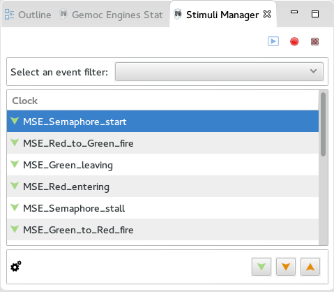
When selecting an MSE you can constrain it by clicking on :
- Green down arrow : no user constraint for this MSE in the next LogicalStep
- Orange down arrow : forbid tick of this MSE in the next LogicalStep. The solver will propose only solutions where this MSE doesn’t tick.
- Orange up : force tick of this MSE in the next LogicalSteps. The solver will propose only solutions where this MSE ticks.
Depending of your choice, the list of proposals will be changed in the Logical Steps view.
Moreover selecting an element in the Logical Steps view will highlight the MSE involved in the Stimuli Manager view.
Tip
This Stimuli Manager view can be used to manually simulate external events.
If defined for a given language, the animation offers some representations of the runtime data. GEMOC supports several ways to add animation to a language.
Important
Animation must not be confused with debug step highlighting that simply highlights the model elements implied in the step that has the focus when the execution is suspended. (In debug, the focus typically depends on the user who selects a step/frame in the Debug view).
Note
if enabled, animation is supposed to be available in both Run and Debug modes.
As seen in Section 3, “Define model animation”, the animation may be provided by several means. The precise procedure to enable/disable it may vary.
If the language provides some animation provided by Sirius (see Section 3.1, “Define an animation representation for Sirius”), then the activation is done via the enabling of dedicated layers.
Note
If the animation service class has been properly configured, then the declared layers will be enabled by default when starting a model execution.
Otherwise, the user may have to enable the layers manually.
Manual enabling/disabling of a layer is usually done by selecting the background of the diagram and then click in the layer drop down command as shown in Figure 19, “Manual activation/deactivation of a Sirius animation layer”.
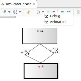
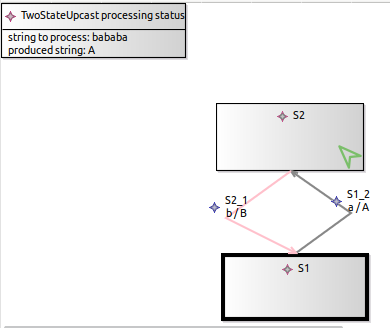
When running, a typical animated visualization of the execution data could be as in Figure 20, “Example of Sirius animation on a FSM DSL.”. In this FSM language, the current state is decorated with a green arrow and a new box shows the buffer content as defined by the language designer in Section 2.1, “Define a debug representation and commands for Sirius”.
By default the Sirius animation will refresh on every engine notification and will wait for the end of the refresh before processing the next steps. While providing precise display, on complex diagram (for example with many queries or several views) this can significantly slow down the model execution speed.
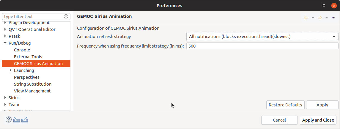
In order to speed up the model execution, GEMOC provides several Sirius animation strategies:
- All notifications: processes all engine diagram refresh notifications. The refresh command is blocking, the model execution is stopped until the refresh is done (slowest)
- Best effort: the refresh is done in a separate job. It uses a single job queue with a discard oldest policy (i.e. the execution continue during the refresh of the diagrams, intermediate notifications may be discarded if the previous refresh hasn’t finished)
- Max frequency limit: use an additional timer in order to guarantee to not call refresh more than the given frequency (default to 500ms)
- Engine pause: the refresh occurs only on the debugger commands (ie. pause / resume / step into / step over …)
- Manual: no automatic refresh, the user has to click on the diagram button to refresh the diagrams (available when selecting the page background in Sirius editors)
These strategies are set in the Preferences → Run/Debug → GEMOC Sirius Animation (see Figure 21, “GEMOC Sirius animation preference page.”)
If the language provides some animation view provided by an Engine addon (see Section 3.2, “Define an animation representation using an engine addon”). The corresponding addon must first be enabled in the launch configuration (see Section 1.2, “Configure engines addons (Frontend/backend)”).
Then, the activation of the language specific representation may vary depending on the addon implementation. Some may provide an Eclipse view that the user has to open, some may popup a new windows.
If the language provides some animation view via semantics calls (see Section 3.3, “Define an animation representation using calls in the semantics”), then the activation of the language specific representation is implementation specific.
Some may simply popup a window, or some may provide an Eclipse view that the user has to open.
They may also require to use a custom parameter passed to the modelInitialization method in the launch configuration.
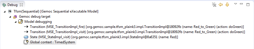
This view is part of the Debug perspective. It presents an interface for Step by Step execution of the model.
When an execution is paused, this view presents a stack containing all ongoing steps, with the last started step at the top of the stack.
At the bottom of the stack is a particular stackframe named Global context.
When selected, this stackframe displays the runtime data in the Variable View.
Note
In order to improve the look and feel in Figure 23, “Debug and Variable views with the sequential engine”, the icons have been customized using the technique described in Section 3.3, “Defining a Concrete Syntax with EMF”
Note
As a language designer, to control how steps should be stacked and presented in the Debug view, consult Section 1.1, “Define model debug step information”.
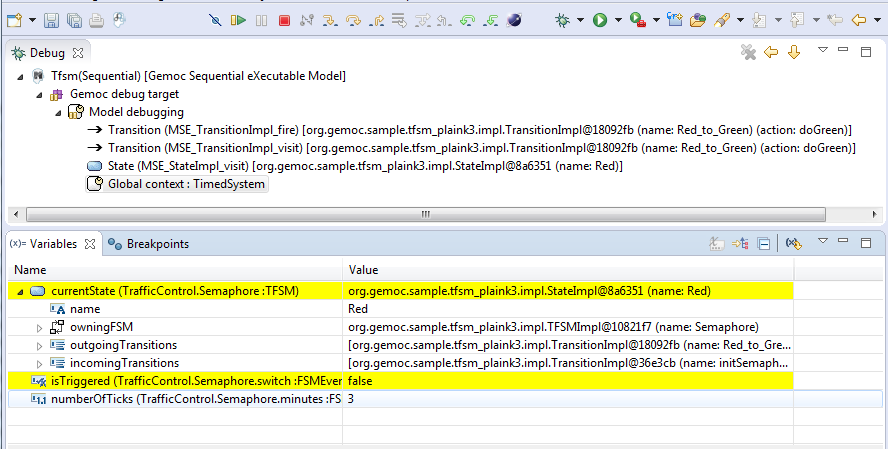
This view is available on the Debug perspective. When an execution is paused, this view presents the current Runtime Data of the model.
Note
As a language designer, to control which Runtime Data should be presented in the Variables view, you need to set
an EAnnotation with nsURI set to aspect on the corresponding EAttributes, EReferences
or EClass in the ecore metamodel. (see Section 1.2, “Define model debug RTD information”).
Tip
When the execution is paused, it is possible to edit the values in this view and then manually change the Runtime Data of the model.
If the MultiDimentional trace is activated, this tip works only if the execution is paused on the last instruction of the trace.
This view is available on the Debug perspective.
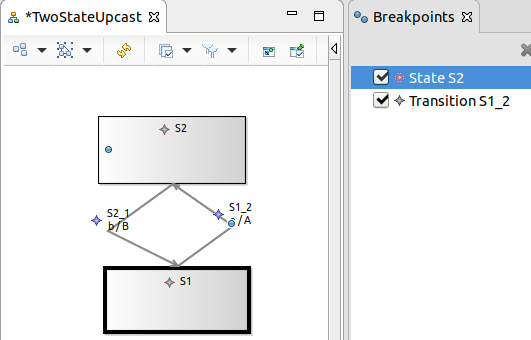
It displays all the breakpoints that have been set for the current execution.
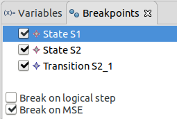
In Figure 22, “Debug view”, the breakpoints listed are ModelElement breakpoints that are linked to model elements in the model (2 States and 1 Transition from K3FSM example). During a model execution in Debug mode, if a DSA is called on one of the elements listed here, then the execution will be suspended.
Note that setting the breakpoints is usually done using Section 3.6, “Editor debug integration”.
GEMOC framework allows to use the classic debug commands Resume, Suspend, Terminate, Step into, Step over, and Step return in order to execute the model.
When paused, the usual debugging tools (step into, step over and step return) can be used to control the execution step by step.
In addition to these commands, if the trace support has been enabled, the execution can also be controlled backward using
the ![]() StepBack Into,
StepBack Into,
![]() StepBack Out and
StepBack Out and
![]() StepBack Over commands.
StepBack Over commands.

When navigating forward and backward, the jump commands offered by the Section 3.5, “Timelines” will be useful too.
The GEMOC Studio features several timeline views that are connected to the trace support. They provide an interactive representation of the execution trace being captured.
This trace support may be either generic or DSL specific (see Section 1.3, “Defining MultiDimentional Trace support”)
Enabling the trace support (and thus the ability to use the timelines) is done in the Engine addons tab of the launch configuration.
Each timeline has its own focus (for example, RunTime Data for the multidimentionnal, or concurrency option decisions for the multibranch) and may have specific limitations on some engines.
The Multidimensional Timeline view provides an interactive representation of the execution trace being captured and the states of the Runtime Data. When double-clicking on a previous state represented in the timeline, the model is brought back into this state. Moreover, the timeline represents all the different runtime data dimensions captured in a trace, each being the sequence of values taken by one specific element of the model. When double-clicking on a value that was reached by an element, the complete model is brought back in the state corresponding to this value. Bullets and line in orange correspond to the current state.
MutiDimensional Timeline Overview. 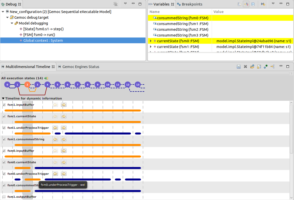
Each bullets on top of the view represent a state of the Runtime Data.
The lines between states represent the method call as a kind of stack. Dot lines indicate that the model has been set back
to a previous state (ie. currently navigating in the past and also represented by the icon
![]() )
)
In this mode, the Debug commands are extended with backward
actions that behave on the call stack similarly to their forward counterparts, but follow
execution steps in the opposite direction:
![]() StepBack Into,
StepBack Into,
![]() StepBack Out, and
StepBack Out, and
![]() StepBack Over.
StepBack Over.
Each row below represent one runtime data dimension. Ie. an attribute or a reference in the model. In these rows, a line indicate that the given data has not changed during these states (Ie. the state has been recorded due to a change in another data)
When exploring the trace, the navigation buttons Navigate backward ![]() Navigate forward
Navigate forward ![]() allows to go directly to the previous or next state
where the given data has changed.
allows to go directly to the previous or next state
where the given data has changed.
The Jump to state ![]() command allows to jump directly to a given state by providing its number.
command allows to jump directly to a given state by providing its number.
The check box at the beginning of each row allows to hide the corresponding data. When unchecked, it is actually put at the bottom of the list.
The state coloration command ![]() allows
to set some unique color on the states using only dimensions that are not hidden.
allows
to set some unique color on the states using only dimensions that are not hidden.
A trace can be saved ![]() and
reloaded
and
reloaded ![]() using the
commands on top of the view. Saved traces can then be compared using the Timeline Diff view or displayed
in the State Graph View.
using the
commands on top of the view. Saved traces can then be compared using the Timeline Diff view or displayed
in the State Graph View.
Note
As the bullets on top of the view represent the Runtime Data states, the number of these will be different from the number of steps that have been executed. (Number of steps executed is displayed in the Engine view)
Tip
Hovering also provides an overview of the data. On a state, it uses the hidden/visible checkbox information to show data only from visible rows.
MutiDimensional Timeline Implicit States. 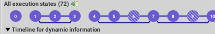
In some cases, like states 6 and 9 in MutiDimensional Timeline Implicit States, some states may use a diagonal hash pattern color. This indicates that some changes in the runtime data have been recorded between 2 declared steps. This can happen for example with nested steps where runtime data are changed in the caller step;
@Step
def public void outerStep() {
... // change some runtime data before calling innerStep()  _self.innerStep()
... // change some runtime data after calling innerStep()
_self.innerStep()
... // change some runtime data after calling innerStep()  }
@Step
def public void innerStep() {
... // change some runtime data
}
@Step
def public void innerStep() {
... // change some runtime data  }
}|
|
change has occurred before the call of inner step; trigger the recording of an implicit state. |
|
|
change has occurred after the call of inner step; trigger the recording of an implicit state. |
|
|
Normal step; trigger the recording of a normal state |
Warning
When going backward then forward again using the Java Engine,
the execution is a kind of replay where only the model is updated. The DSA
operations are not run.
The DSA will run again normally when the engine will try to run the last recorded
Step in the timeline.
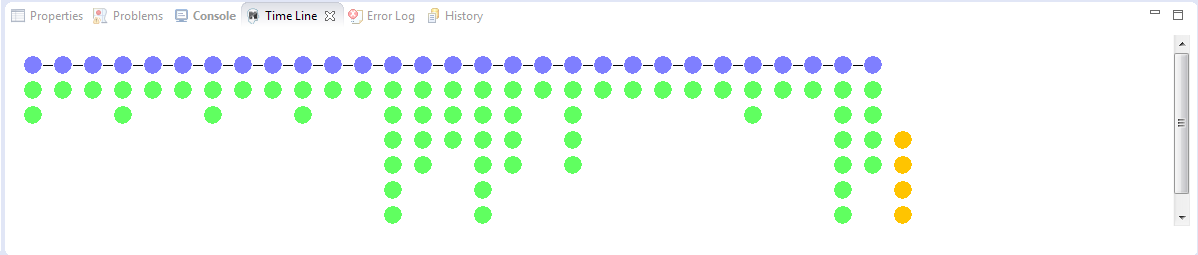
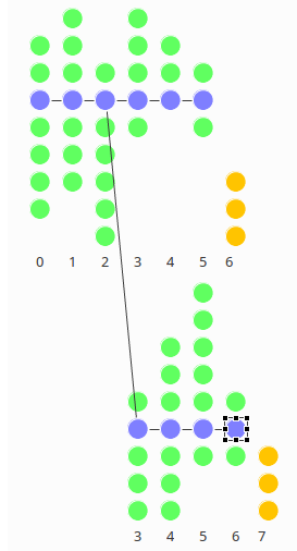
Formerly known as Event Scheduling Timeline view, this view represents the lines of the model’s execution with a focus for concurrent behavior and LogicalSteps events. It displays:
- the different logical steps proposed by the solver in the past in blue color,
- the selected logical steps at each execution step in green color,
- and the possible future logical steps in yellow color,
- the model specific events for each logical step.
Note
This view can be enabled/disabled in the launch configuration by checking "Execution tracing" in the Engine Addons tab.
Note
The possible future logical steps are shown under the condition that the model is executing.
In addition to displaying information, it also provides interaction with the user. During execution, it is possible to come back into the past by double-clicking on any of the blue logical steps. It does three things:
- it resets the solver’s state to the selected execution step,
- and it resets the model’s state to the selected execution step,
- it also forks the current timeline and create a new branch of execution.
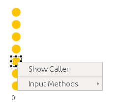
It is also possible to select a logical step and use the contextual menu to show its caller in the Sirius editor:
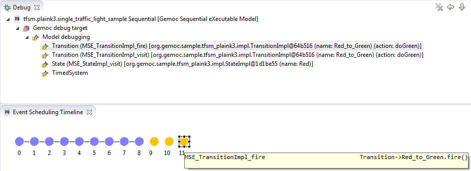
As the Java engine doesn’t offer execution branches (no possible concurrent actions), all commands related to branches are disabled and the timeline will allow to display only a straight line.
Warning
When going backward then forward again using the Java Engine,
the execution is a kind of replay where only the model is updated. The DSA
operations are not run.
The DSA will run again normally when the engine will try to run the last recorded
Step in the timeline.
This view allows to compare the Runtime Data dimensions of two saved traces.
Obtaining traces can be done using the save command in the Section 3.5.1, “Multidimentional timeline view”.
This view allows to search for cycles in the current trace.
This view is synchronized with the Section 3.5.1, “Multidimentional timeline view” and uses the hide/show dimension checkboxes information in order to display the state graph only for visible data.
If you have defined a debug representation using Section 2.1, “Define a debug representation and commands for Sirius”. You can use the following actions to start a debug session and toggle breakpoints.
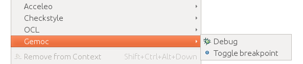
Usually, elements with a break point are decorated with a blue bullet.
Additionally, when suspended during the execution in Debug mode, the target of the current instruction in the call stack can be highlighted. In the following example, (Figure 27, “Sirius debug stack highlighting”) the selected element in the Debug stack (top left) is highlighted in yellow in Sirius (bottom left) thanks to the Debug layer added to the editor.
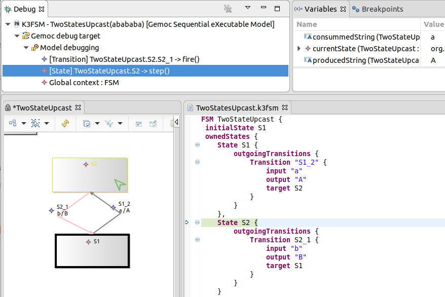
If your language has a concrete syntax specified using XText, when running a model, the debugger will take care to highlight the correct line in the xtext editor corresponding to the target model element of the selected call in the call stack.
In the following example, (Figure 28, “Xtext debug stack highlighting”) the selected element in the Debug stack (top left) is highlighted with an arrow in Xtext (bottom right).

[32] asciidoc source of this page: https://github.com/eclipse/gemoc-studio/tree/master/docs/org.eclipse.gemoc.studio.doc/src/main/asciidoc/userguide/mw_ExecuteAnimateDebug_headContent.asciidoc.
[33] asciidoc source of this page: https://github.com/eclipse/gemoc-studio/tree/master/docs/org.eclipse.gemoc.studio.doc/src/main/asciidoc/userguide/mw_ExecuteModel_headContent.asciidoc.
[34] asciidoc source of this page: https://github.com/eclipse/gemoc-studio-modeldebugging/tree/master/java_execution/java_engine/plugins/org.eclipse.gemoc.execution.sequential.javaengine.ui/docs/asciidoc/user_mw_LaunchSequentialModelExecution.asciidoc.
[35] asciidoc source of this page: https://github.com/eclipse/gemoc-studio/tree/master/docs/org.eclipse.gemoc.studio.externaltools.doc/src/main/asciidoc/ccsljavaxdsml/user_mw_LaunchConcurrentModelExecution.asciidoc.
[36] asciidoc source of this page: https://github.com/eclipse/gemoc-studio/tree/master/docs/org.eclipse.gemoc.studio.doc/src/main/asciidoc/userguide/mw_ConfigureEngineAddons.asciidoc.
[37] asciidoc source of this page: https://github.com/eclipse/gemoc-studio-modeldebugging/tree/master/framework/execution_framework/plugins/org.eclipse.gemoc.executionframework.ui/docs/asciidoc/user_mw_EngineView.asciidoc.
[38] asciidoc source of this page: https://github.com/eclipse/gemoc-studio/tree/master/docs/org.eclipse.gemoc.studio.externaltools.doc/src/main/asciidoc/ccsljavaxdsml/user_mw_EngineView_ccsljava_addition.asciidoc.
[39] asciidoc source of this page: https://github.com/eclipse/gemoc-studio/tree/master/docs/org.eclipse.gemoc.studio.externaltools.doc/src/main/asciidoc/ccsljavaxdsml/user_mw_ControlModelExecution_LogicalStepView.asciidoc.
[40] asciidoc source of this page: https://github.com/eclipse/gemoc-studio/tree/master/docs/org.eclipse.gemoc.studio.externaltools.doc/src/main/asciidoc/ccsljavaxdsml/user_mw_ControlModelExecution_StimuliManagerView.asciidoc.
[41] asciidoc source of this page: https://github.com/eclipse/gemoc-studio/tree/master/docs/org.eclipse.gemoc.studio.doc/src/main/asciidoc/userguide/mw_AnimateModel_headContent.asciidoc.
[42] asciidoc source of this page: https://github.com/eclipse/gemoc-studio-modeldebugging/tree/master/framework/xdsml_framework/plugins/org.eclipse.gemoc.xdsmlframework.extensions.sirius/docs/asciidoc/user_mw_AnimateModel_using_sirius.asciidoc.
[43] asciidoc source of this page: https://github.com/eclipse/gemoc-studio/docs/org.eclipse.gemoc.studio.doc/src/main/asciidoc/userguide/mw_AnimateModel_using_engine_addon.asciidoc.
[44] asciidoc source of this page: https://github.com/eclipse/gemoc-studio/docs/org.eclipse.gemoc.studio.doc/src/main/asciidoc/userguide/mw_AnimateModel_using_engine_addon.asciidoc.
[45] asciidoc source of this page: https://github.com/eclipse/gemoc-studio-modeldebugging/tree/master/framework/execution_framework/plugins/org.eclipse.gemoc.executionframework.debugger.ui/docs/acsiidoc/user_mw_DebugModel_DebugView.asciidoc.
[46] asciidoc source of this page: https://github.com/eclipse/gemoc-studio-modeldebugging/tree/master/framework/execution_framework/plugins/org.eclipse.gemoc.executionframework.debugger.ui/docs/acsiidoc/user_mw_DebugModel_VariablesView.asciidoc.
[47] asciidoc source of this page: https://github.com/eclipse/gemoc-studio-modeldebugging/tree/master/framework/execution_framework/plugins/org.eclipse.gemoc.executionframework.debugger.ui/docs/acsiidoc/user_mw_DebugModel_BreakpointsView.asciidoc.
[48] asciidoc source of this page: https://github.com/eclipse/gemoc-studio-modeldebugging/tree/master/framework/execution_framework/plugins/org.eclipse.gemoc.executionframework.debugger.ui/docs/acsiidoc/user_mw_DebugModel_DebugCommands.asciidoc.
[49] asciidoc source of this page: https://github.com/eclipse/gemoc-studio/tree/master/docs/org.eclipse.gemoc.studio.doc/src/main/asciidoc/userguide/mw_DebugModel_Timelines_headContent.asciidoc.
[50] asciidoc source of this page: https://github.com/eclipse/gemoc-studio-modeldebugging/tree/master/trace/manager/plugins/org.eclipse.gemoc.addon.multidimensional.timeline/docs/asciidoc/user_mw_DebugModel_MultiDimentionalTimeline.asciidoc.
[51] asciidoc source of this page: https://github.com/eclipse/gemoc-studio-modeldebugging/tree/master/java_execution/java_engine/plugins/org.eclipse.gemoc.execution.sequential.javaengine.ui/docs/asciidoc/user_mw_DebugModel_MultiDimentionalTimeline_javaengine.asciidoc.
[52] asciidoc source of this page: https://github.com/eclipse/gemoc-studio/tree/master/docs/org.eclipse.gemoc.studio.externaltools.doc/src/main/asciidoc/ccsljavaxdsml/user_mw_DebugModel_MultiBranchTimeline.asciidoc.
[53] asciidoc source of this page: https://github.com/eclipse/gemoc-studio-modeldebugging/tree/master/java_execution/java_engine/plugins/org.eclipse.gemoc.execution.sequential.javaengine.ui/docs/asciidoc/user_mw_DebugModel_MultiDimentionalTimeline_javaengine.asciidoc.
[54] asciidoc source of this page: https://github.com/eclipse/gemoc-studio-modeldebugging/tree/master/trace/manager/plugins/org.eclipse.gemoc.addon.diffviewer/docs/asciidoc/user_mw_DebugModel_Timeline_diff_view.asciidoc.
[55] asciidoc source of this page: https://github.com/eclipse/gemoc-studio-modeldebugging/tree/master/trace/manager/plugins/org.eclipse.gemoc.addon.stategraph/docs/asciidoc/user_mw_DebugModel_Timeline_state_graph_view.asciidoc.
